Visualize your data with ggplot
2025-10-10
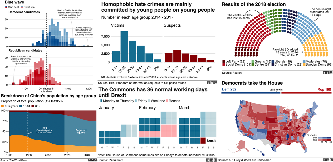
Graphs
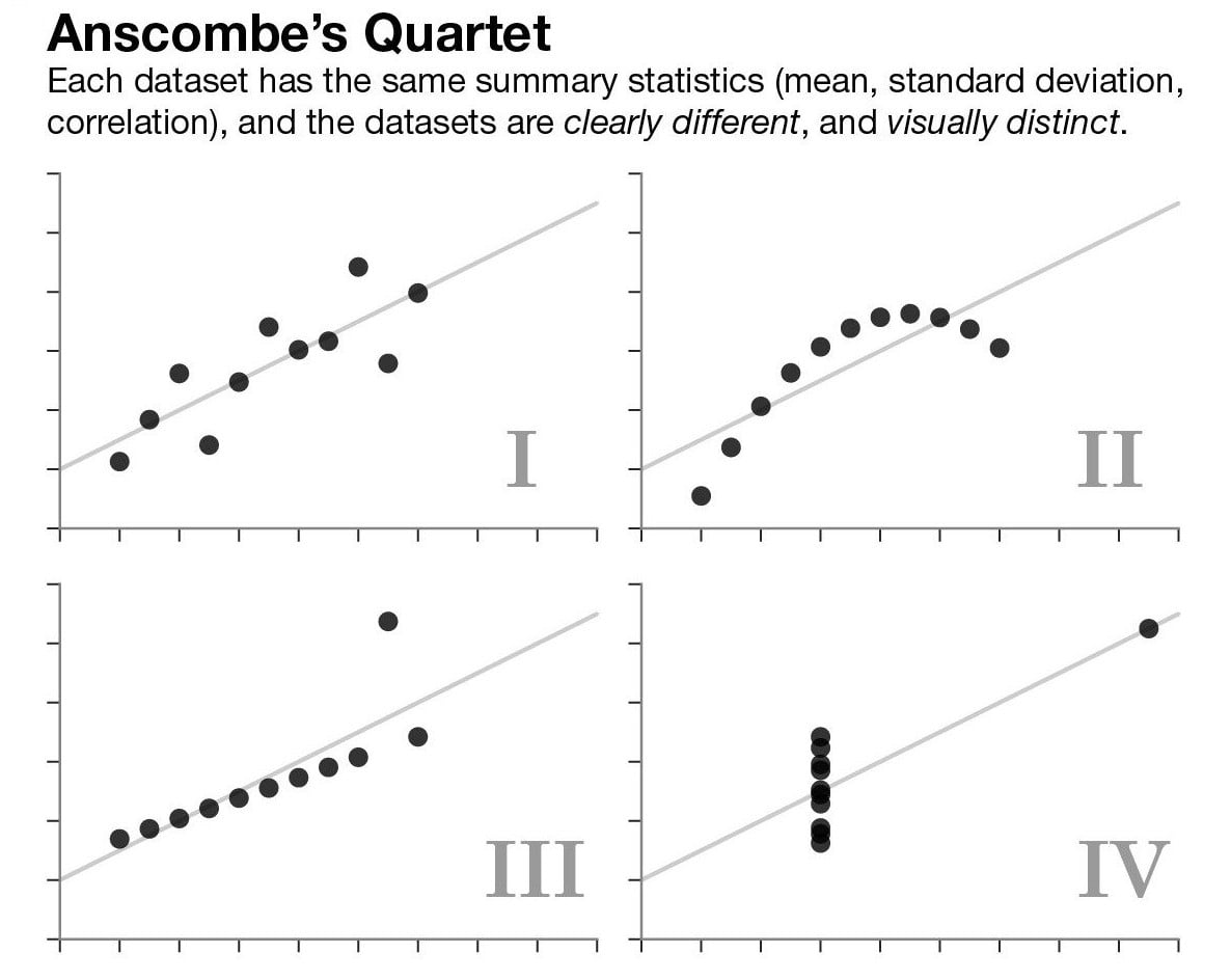
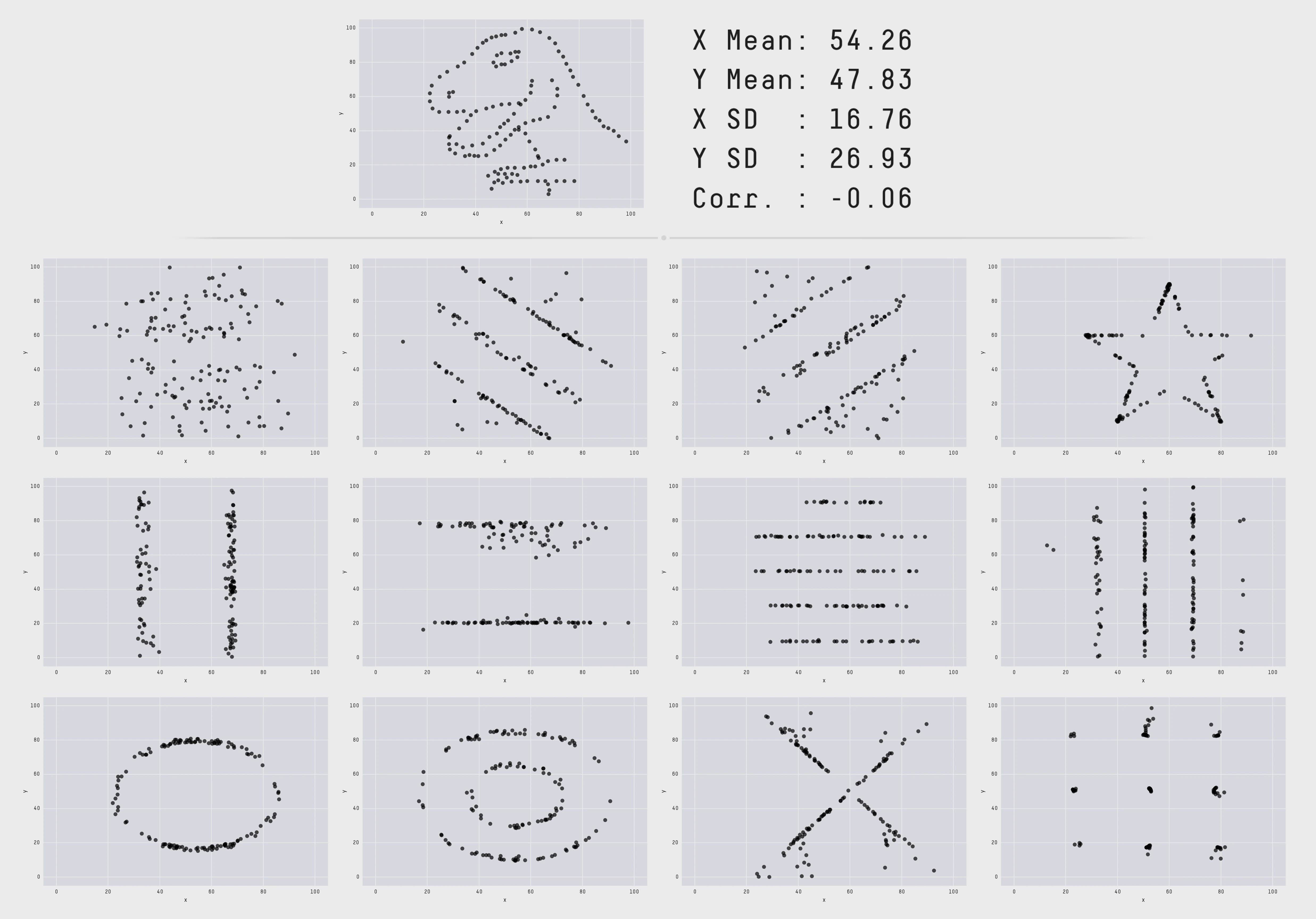
Essentialpart of data analyses
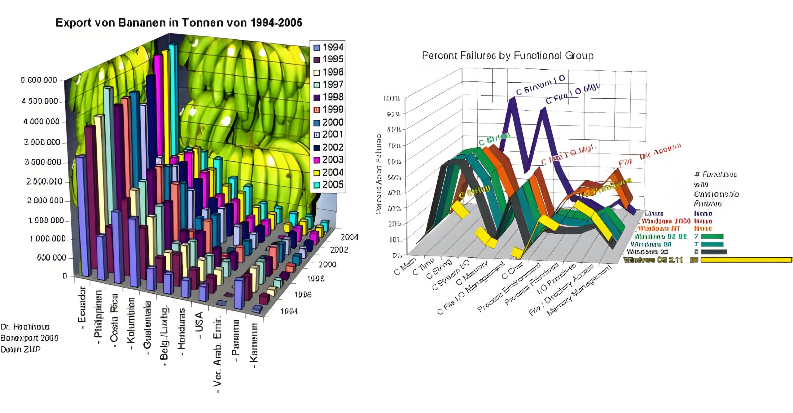
- Data with
same summary statisticscan look verydifferent when plottedout.
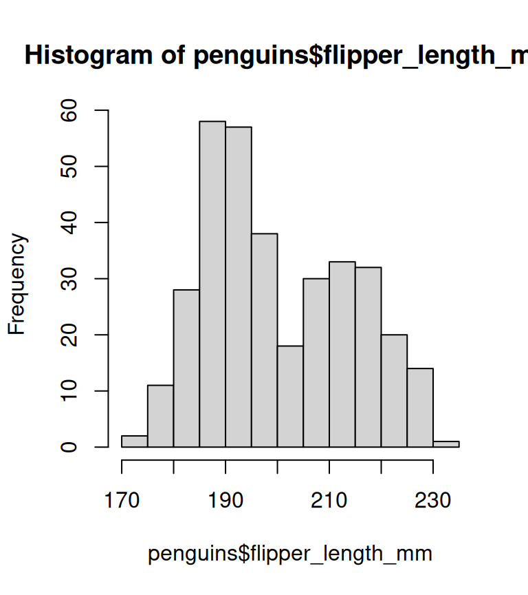
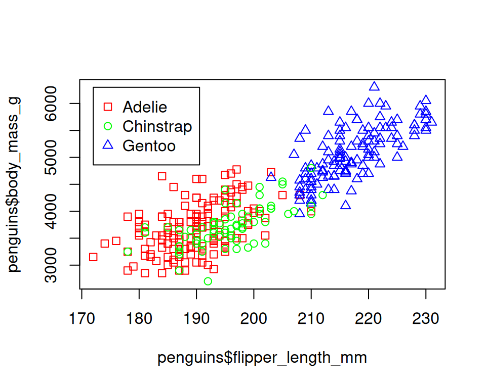
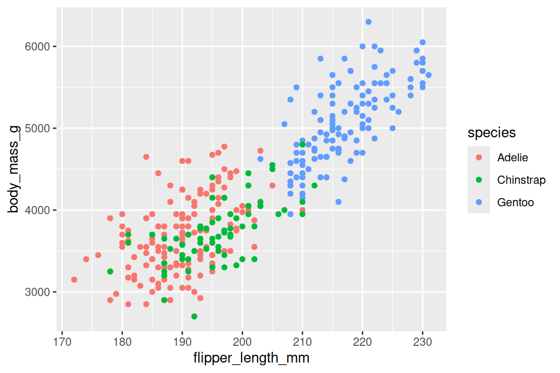
Base Graphics vs ggplot2
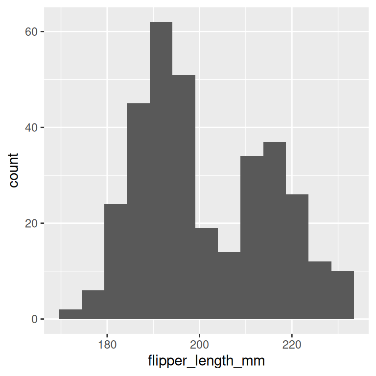
Base Graphics vs ggplot2
basic r plot
Grammar Of Graphics
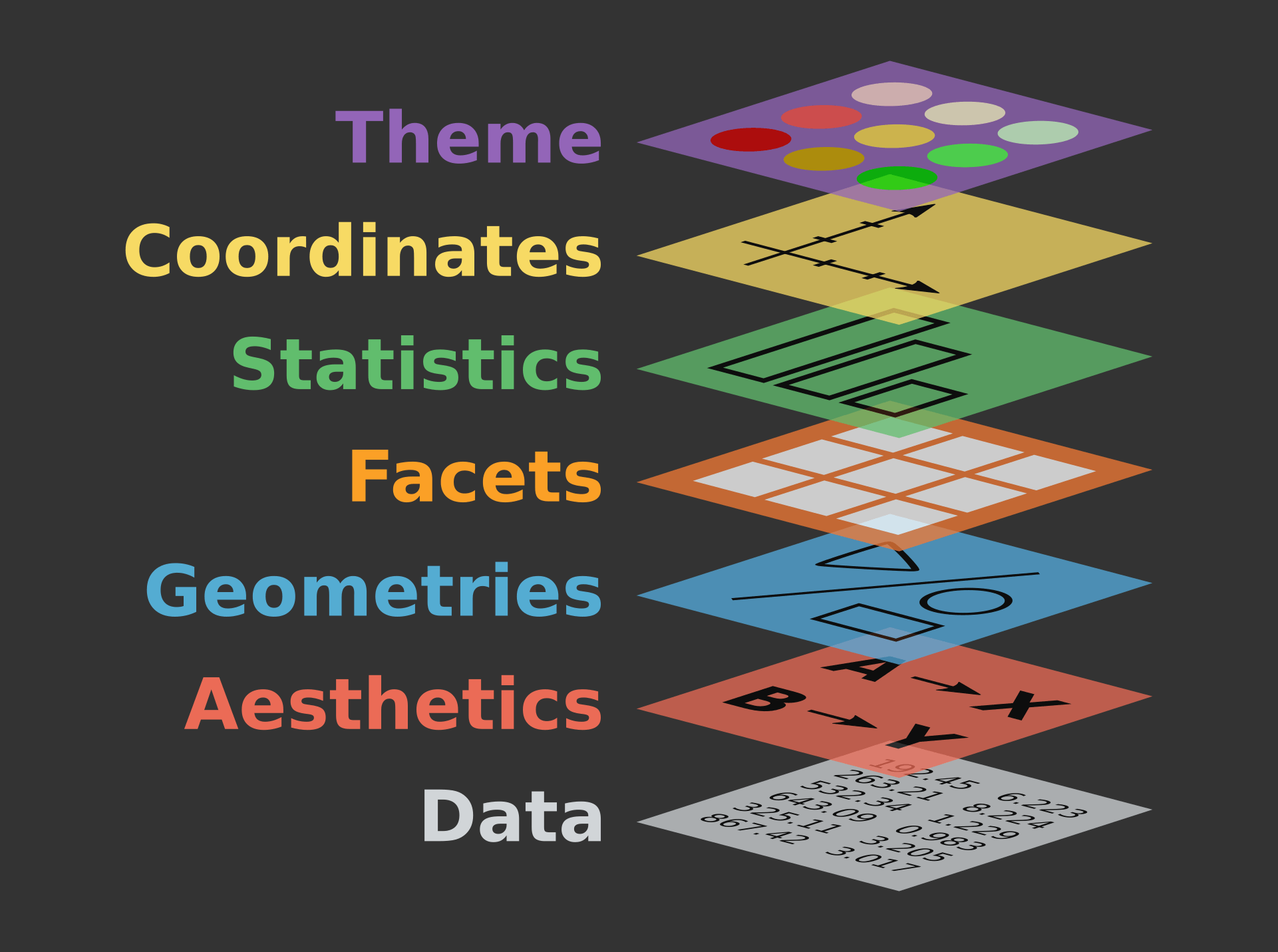
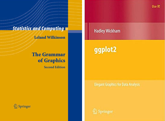
- Leland Wilkinson’s The Grammar of Graphics
- Created by Hadley Wickham in 2005
- Data: Input data.
Table, csv, xlsx - Aesthetic: Mapping or visual characteristics of the geometry.
Size, Color, Shapeetc - Geometries: A geometry representing data.
Points, Linesetc - Facets: Split plot into
subplot - Statistics: Statistical transformations.
Counts, Meansetc - Coordinates: Numeric system to determine position of geometry.
Cartesian, Polaretc - Scale: How visual characteristics are converted to display values
- Theme: controls points of display.
Font size, background colour
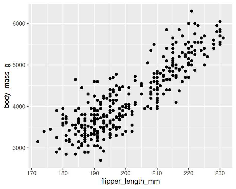
Building A Graph: • Syntax
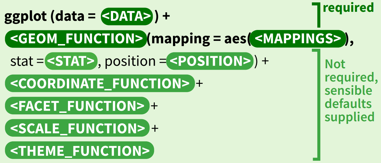
Building A Graph
![]()

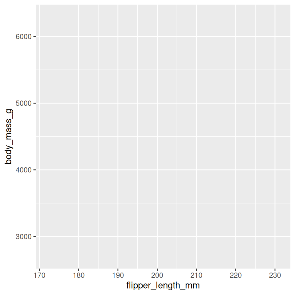
Building A Graph

Building A Graph
Building A Graph
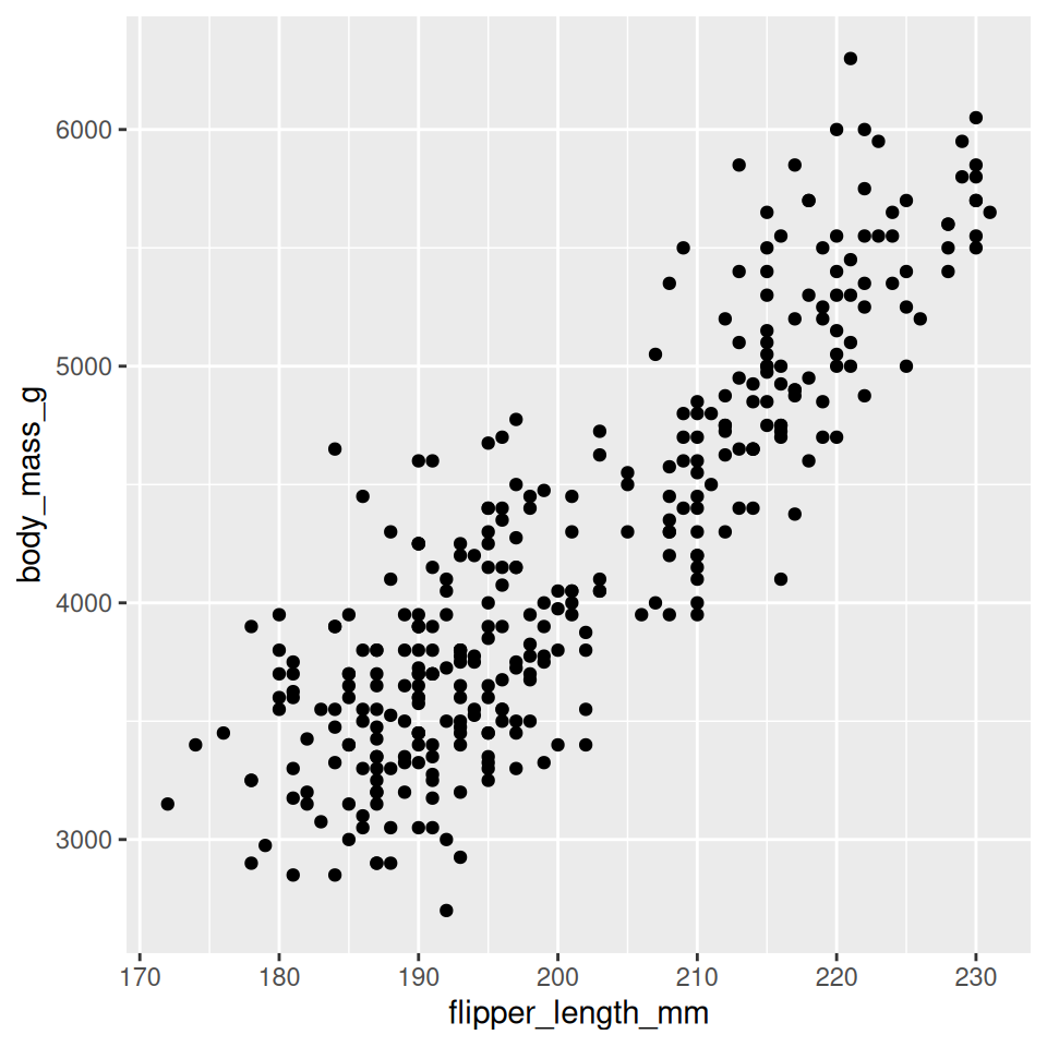
Building A Graph

Building A Graph
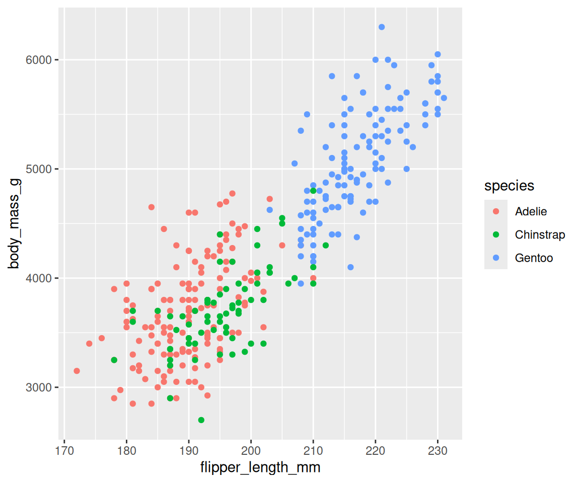
Building A Graph

Data • format
- Transforming data into ‘long’ or ‘wide’ formats
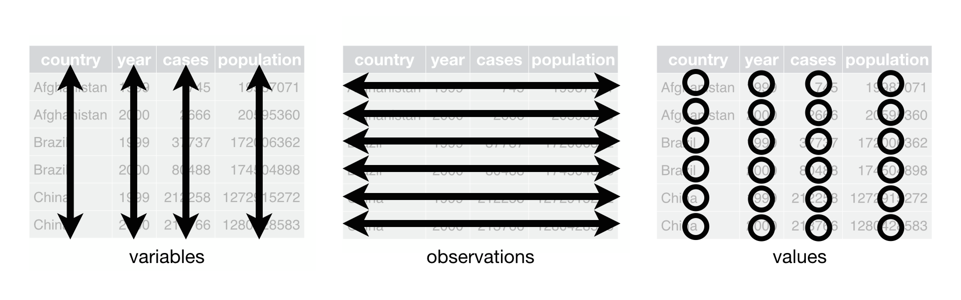
Wide
# A tibble: 4 × 8
  species island    bill_length_mm bill_depth_mm flipper_length_mm body_mass_g
  <fct>   <fct>              <dbl>         <dbl>             <int>       <int>
1 Adelie  Torgersen           39.1          18.7               181        3750
2 Adelie  Torgersen           39.5          17.4               186        3800
3 Adelie  Torgersen           40.3          18                 195        3250
4 Adelie  Torgersen           NA            NA                  NA          NA
# ℹ 2 more variables: sex <fct>, year <int>
Long
species island sex year variables value
1 Adelie Torgersen male 2007 bill_length_mm 39.1
2 Adelie Torgersen male 2007 bill_depth_mm 18.7
3 Adelie Torgersen male 2007 flipper_length_mm 181.0
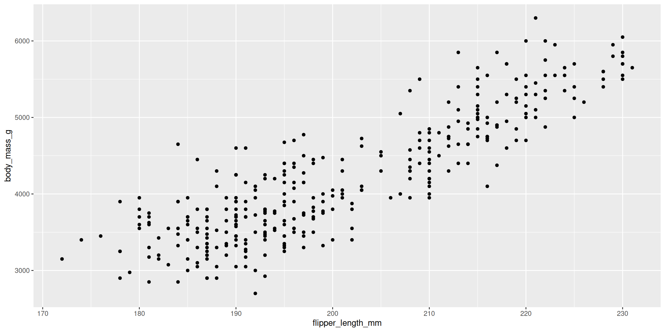
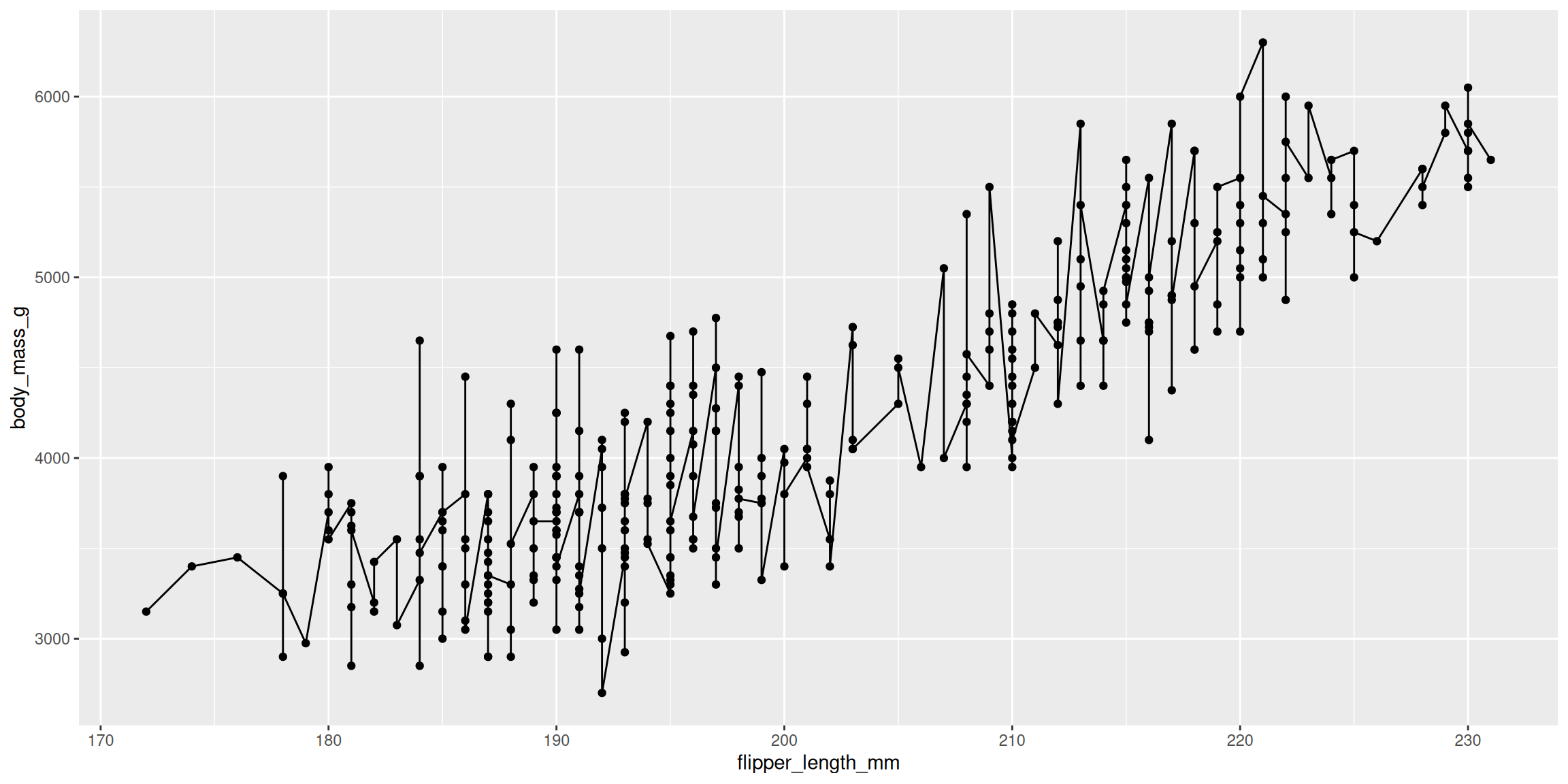
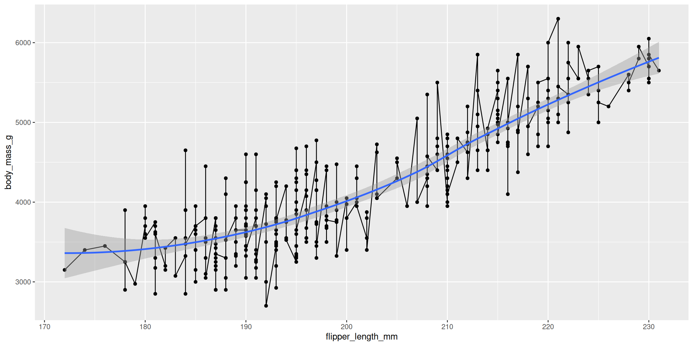
4 Adelie Torgersen male 2007 body_mass_g 3750.0Geoms • types
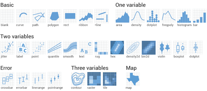
Stats
Statscompute new variables from input data.Geomshave default stats.- Plots can be built with stats.

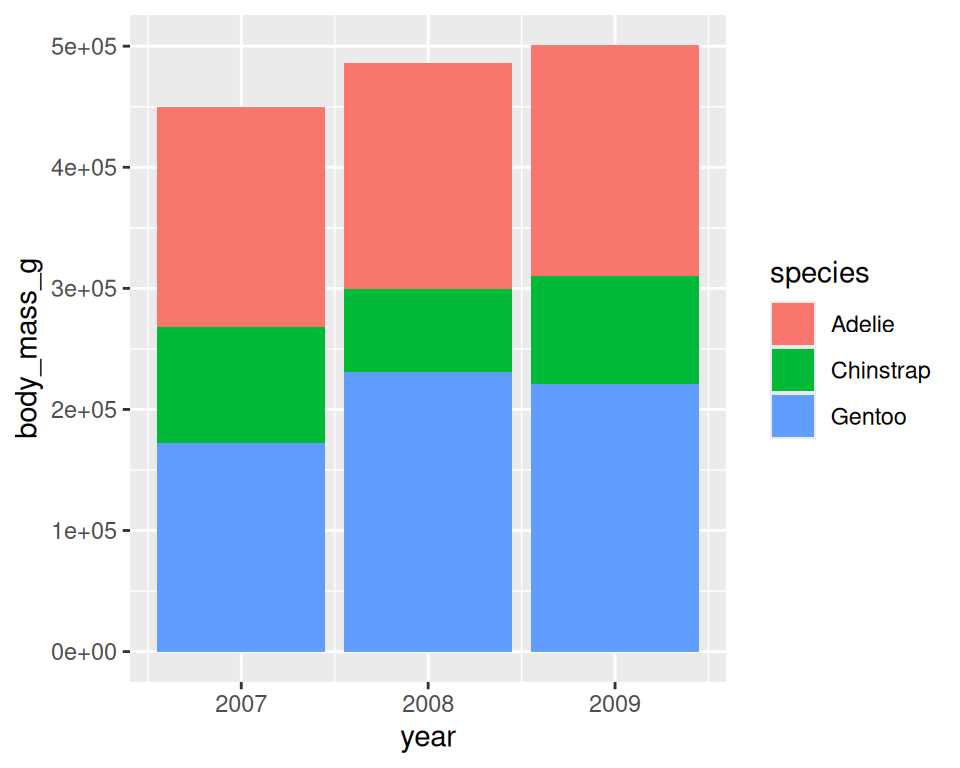
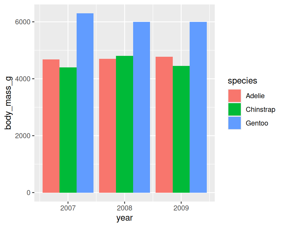
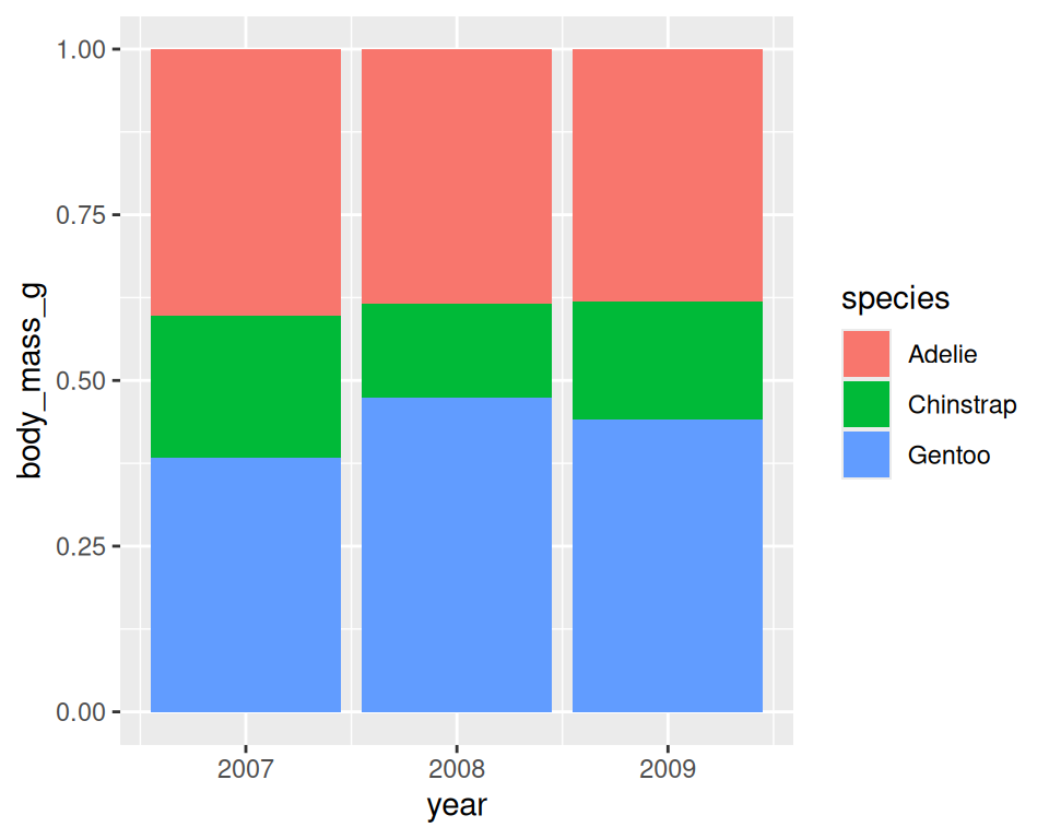
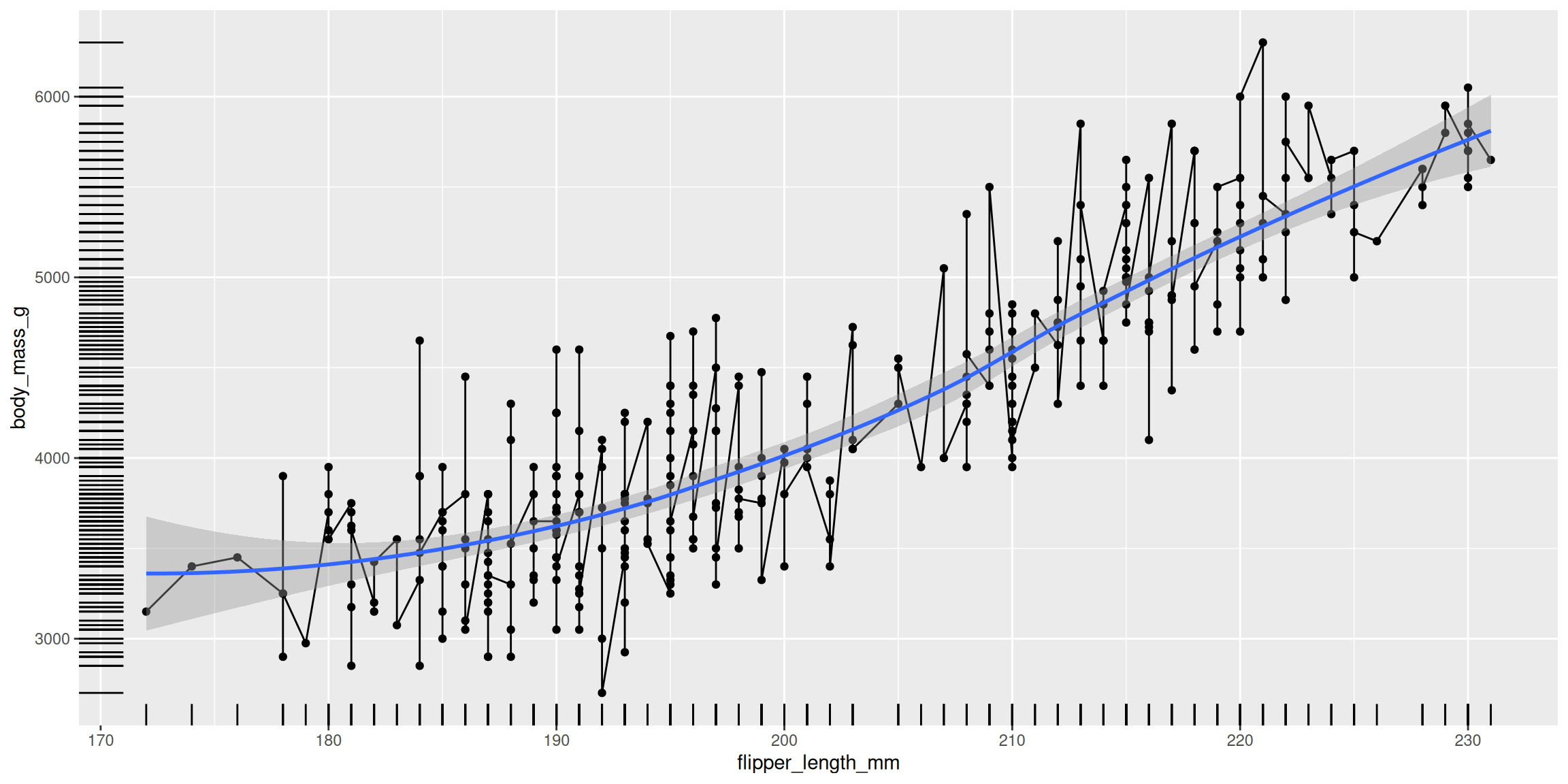
Position
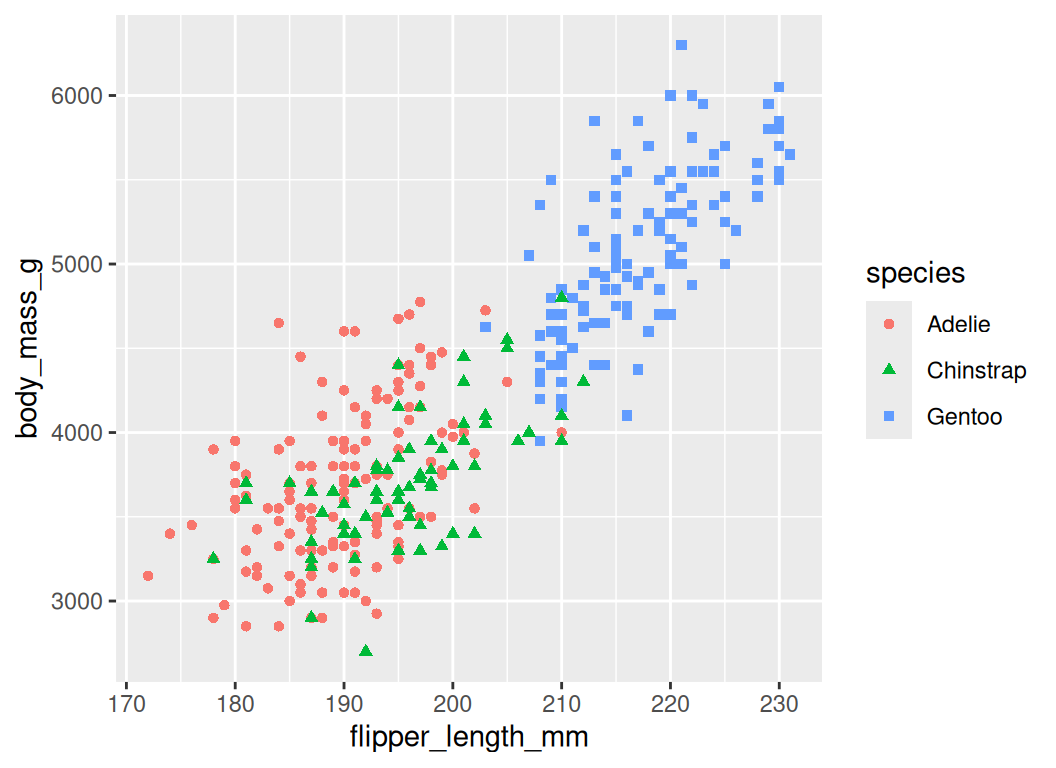
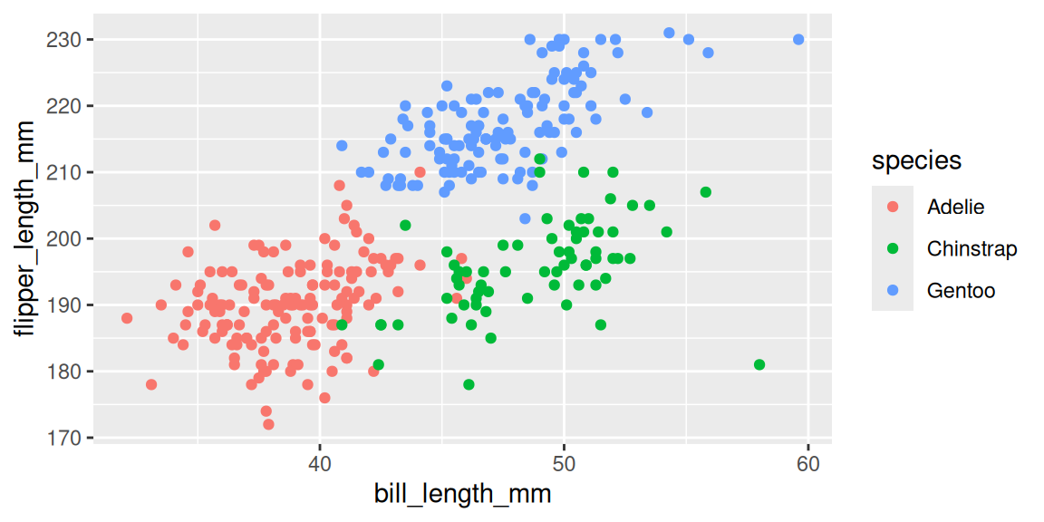
Aesthetics
- Aesthetic
mapping
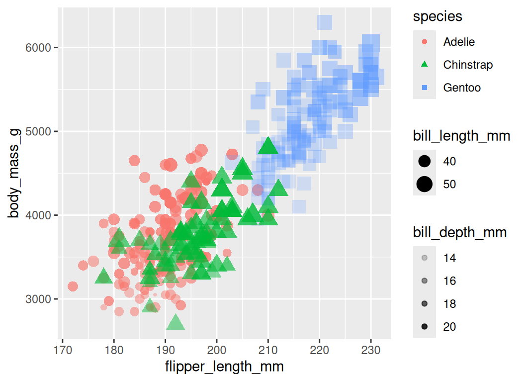
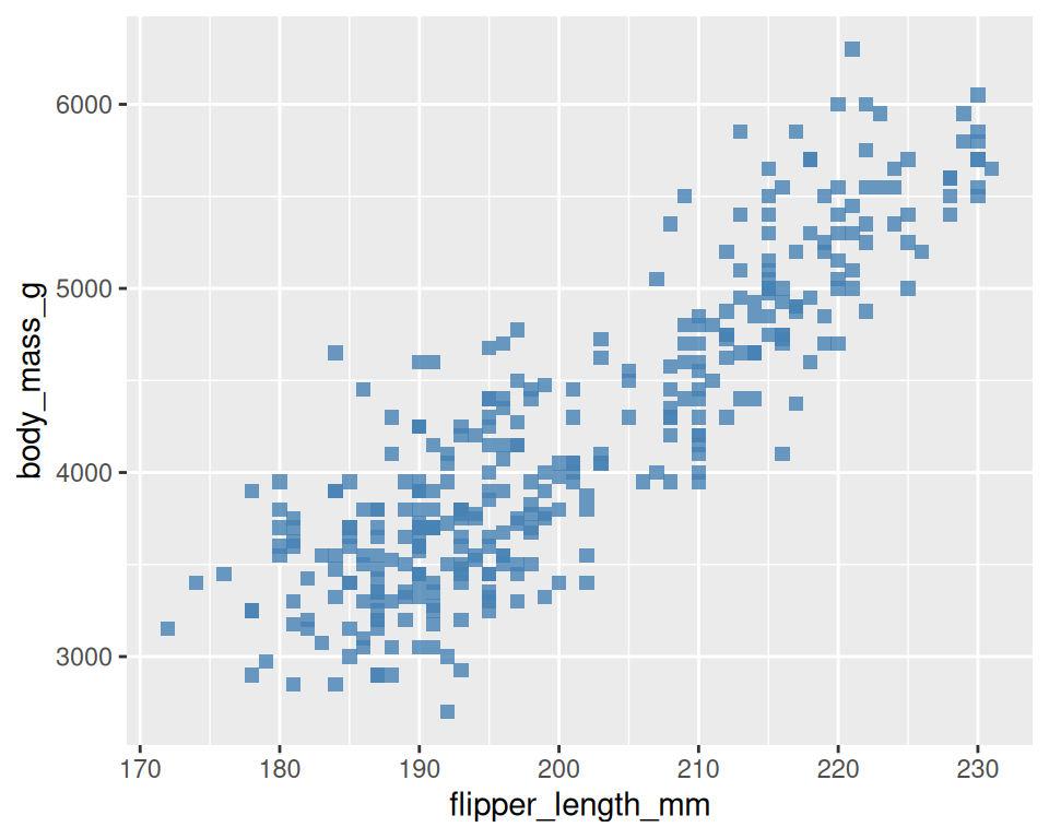
Aesthetics
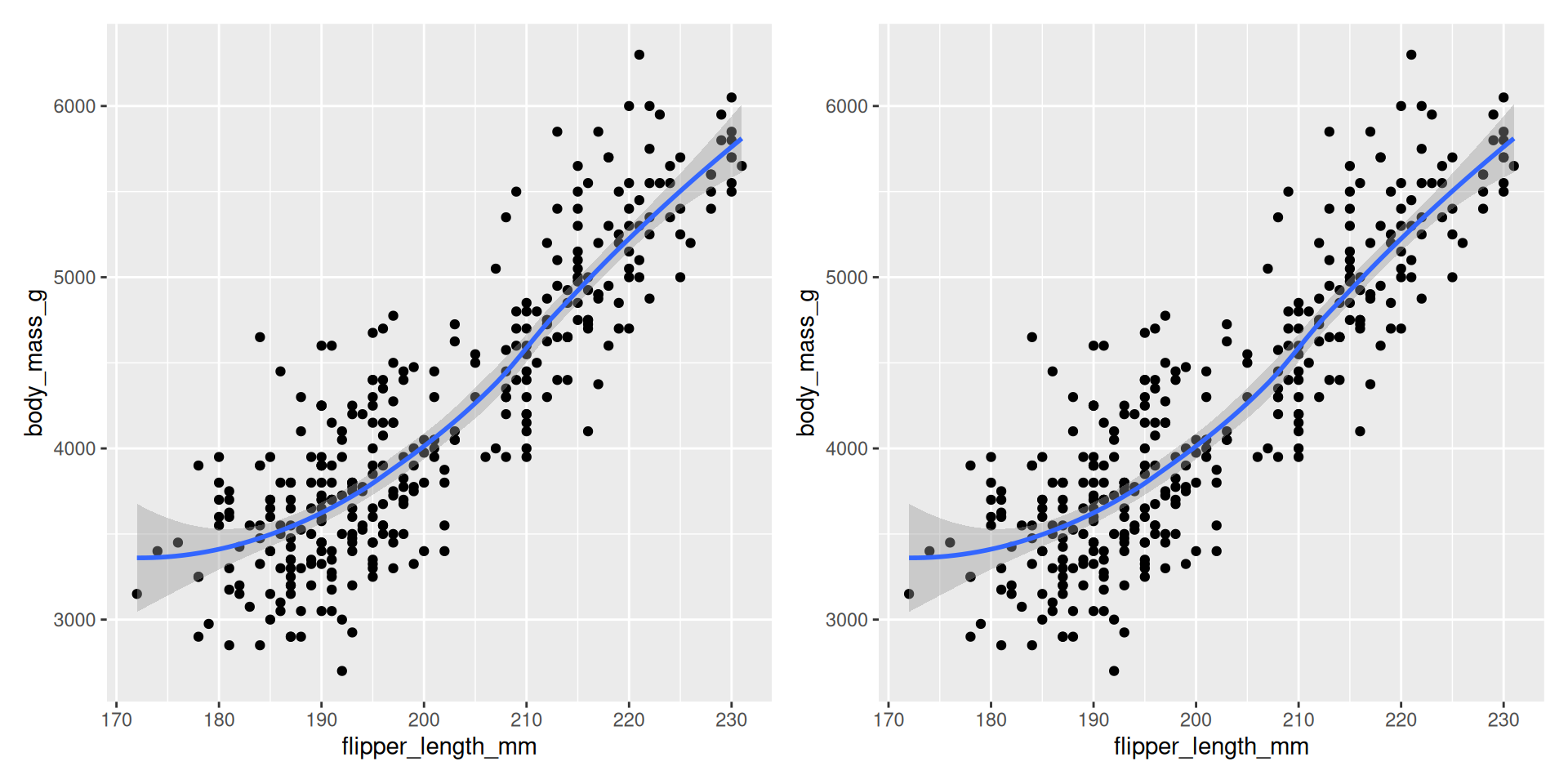
Multiple Geoms
Multiple Geoms
Multiple Geoms
Multiple Geoms
Multiple Geoms

Multiple Geoms
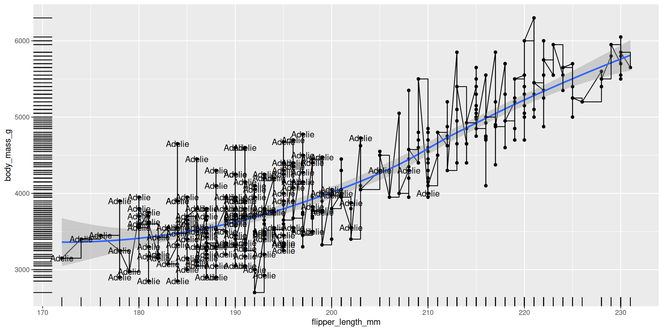
Just because you can doesn’t mean you should!
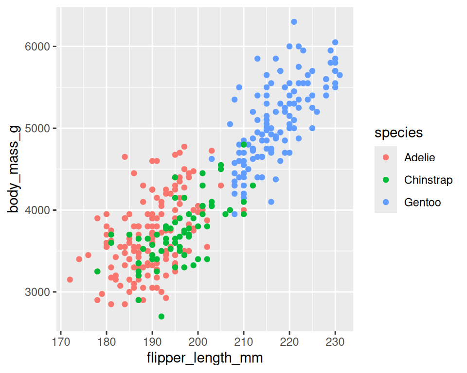
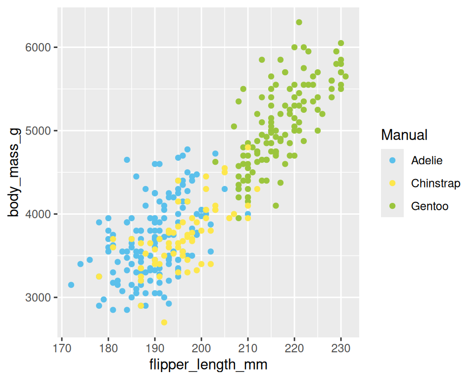
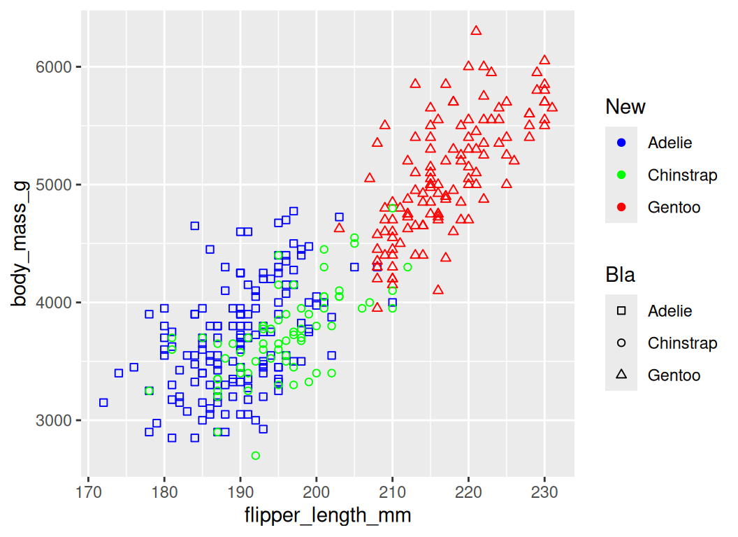
Scales • Discrete Colors
- scales: position, color, fill, size, shape, alpha, linetype
- syntax:
scale_<aesthetic>_<type>
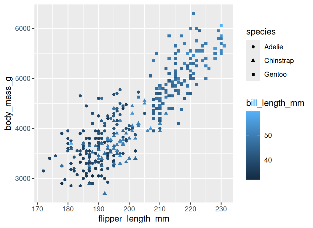
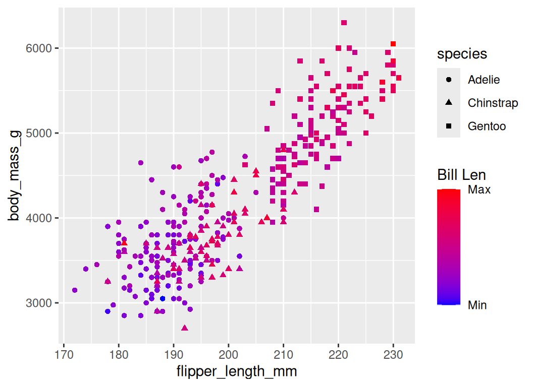
Scales • Continuous Colors
- In RStudio, type
scale_, then press TAB
Scales • Shape
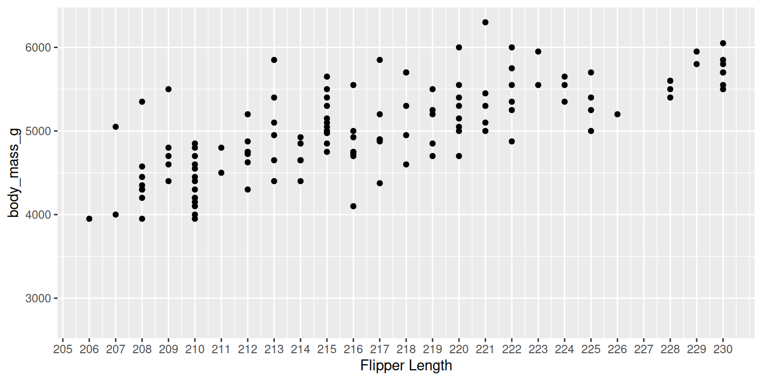
Scales • Axes
- scales: x, y
- syntax:
scale_<axis>_<type> - arguments: name, limits, breaks, labels
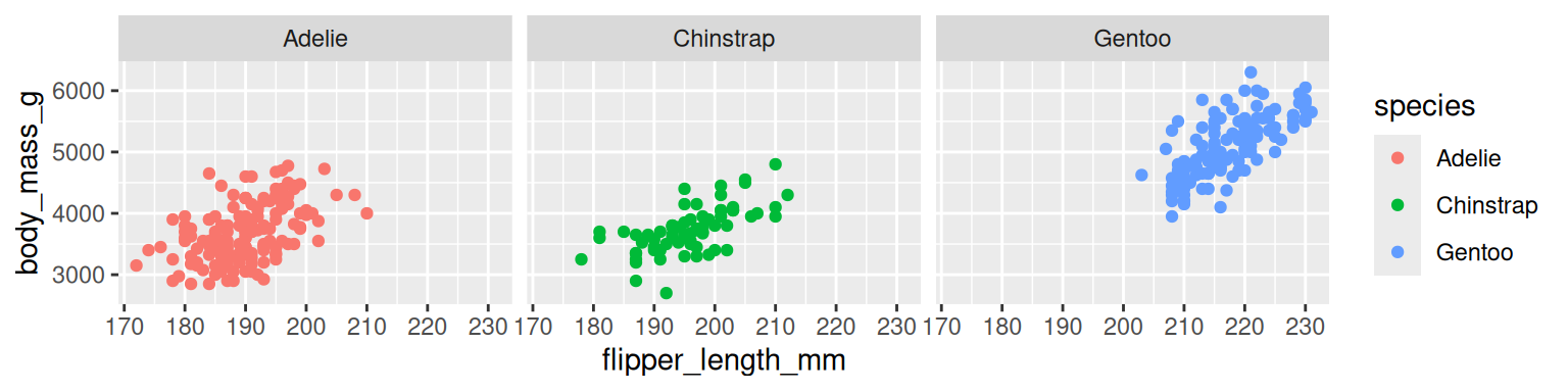
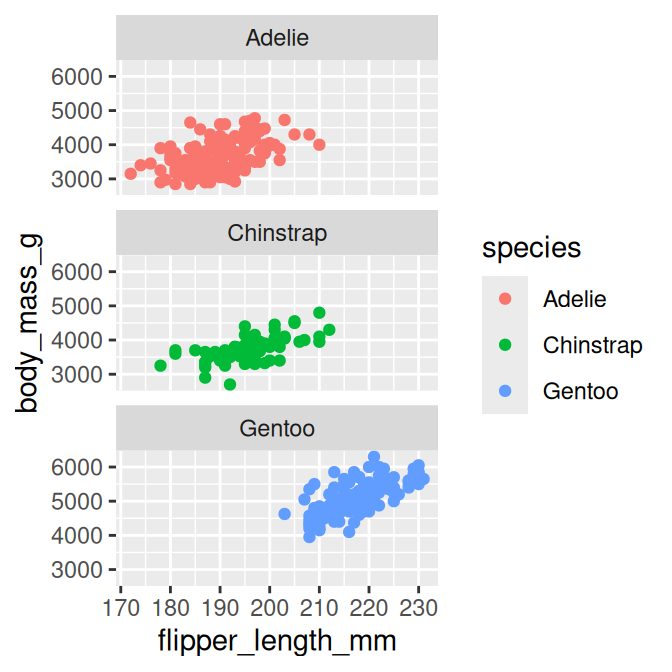
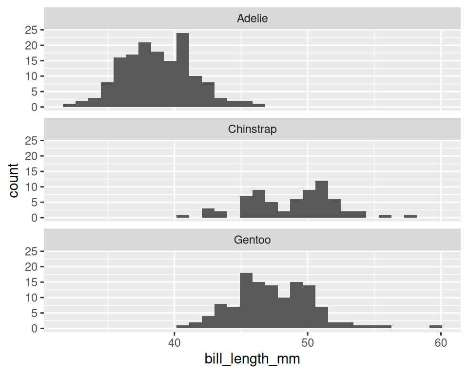
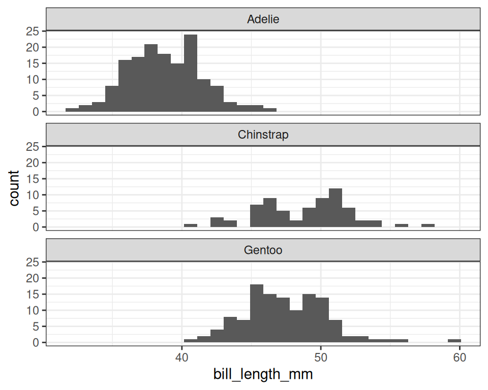
Facets • facet_wrap
Split to subplotsbased on variable(s),- Faceting in
one dimension

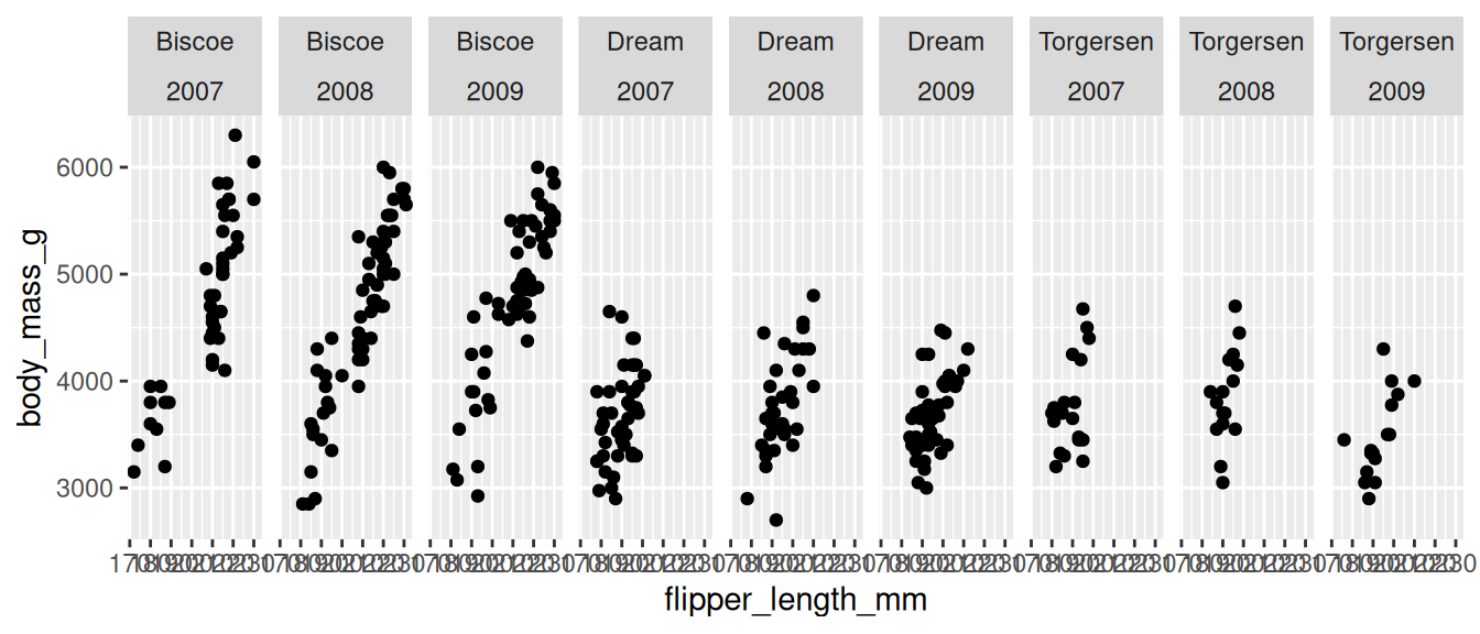
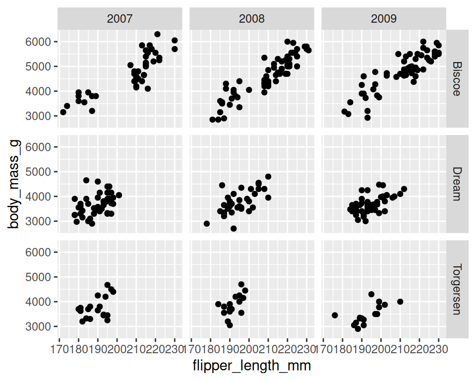
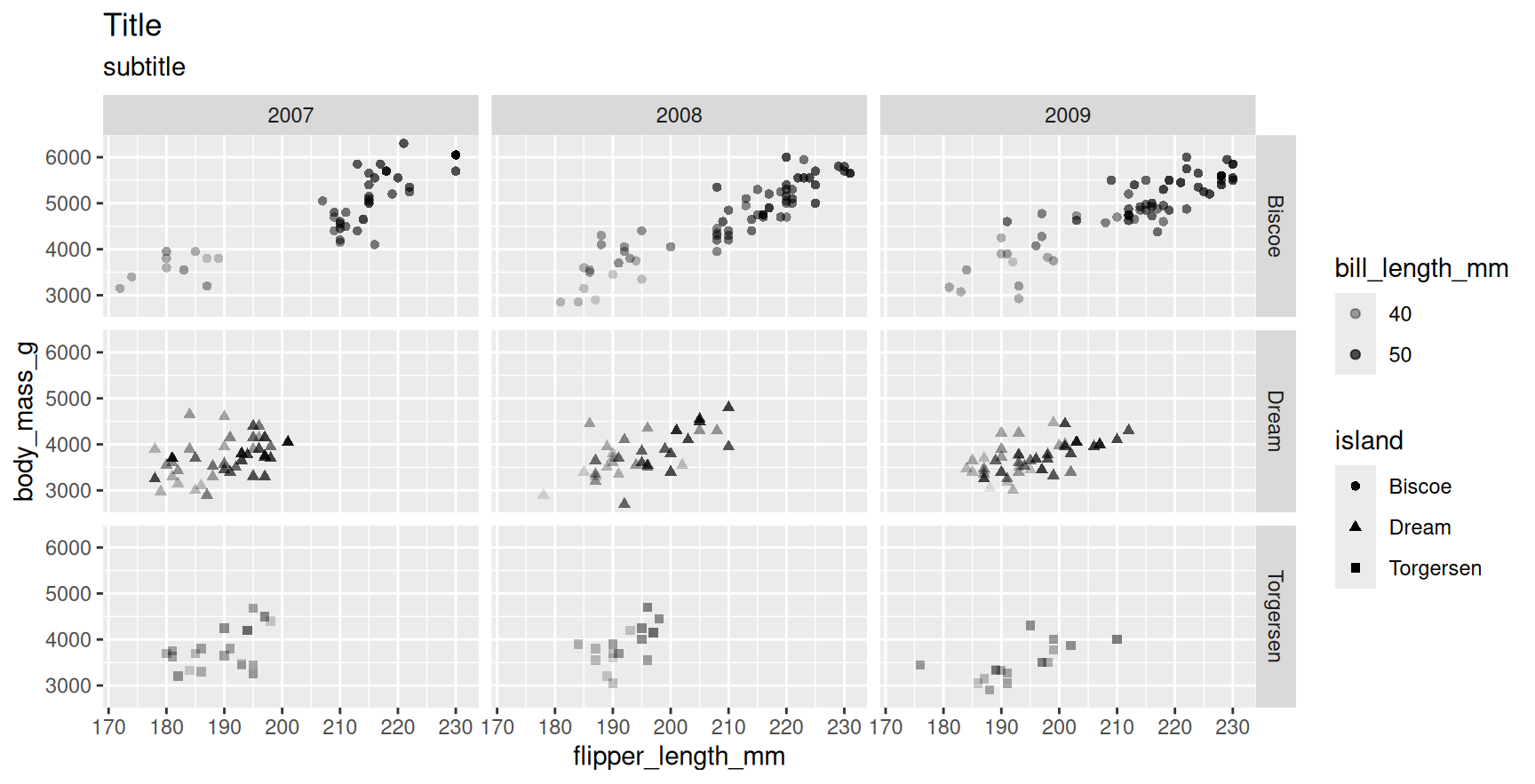
Facets • facet_grid
- Faceting in
two dimensions
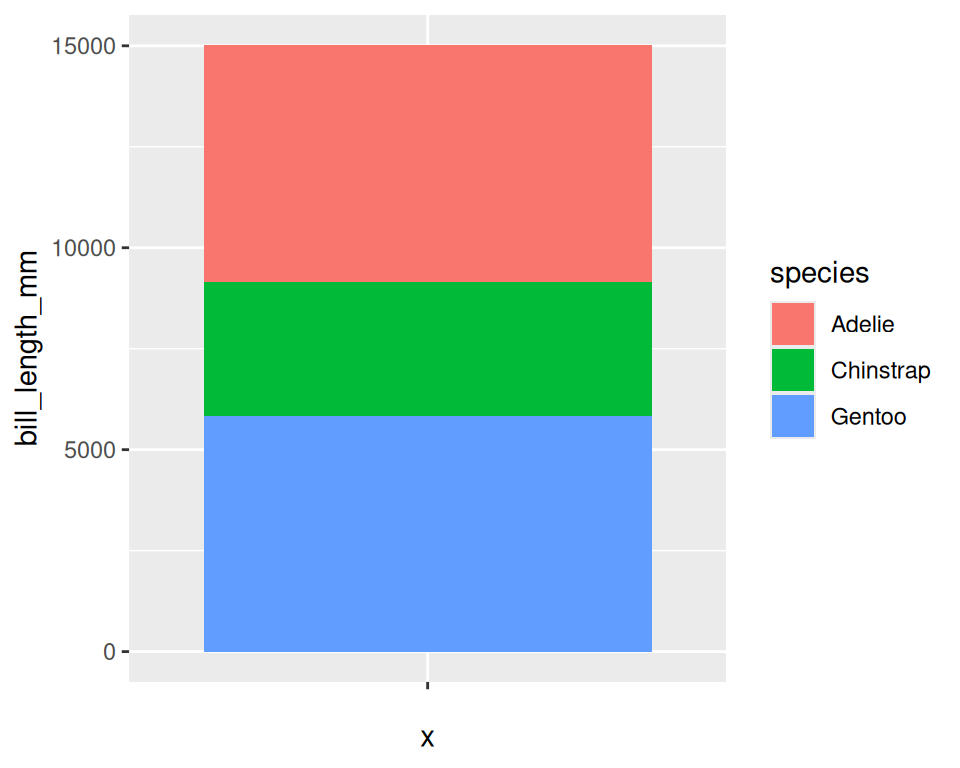
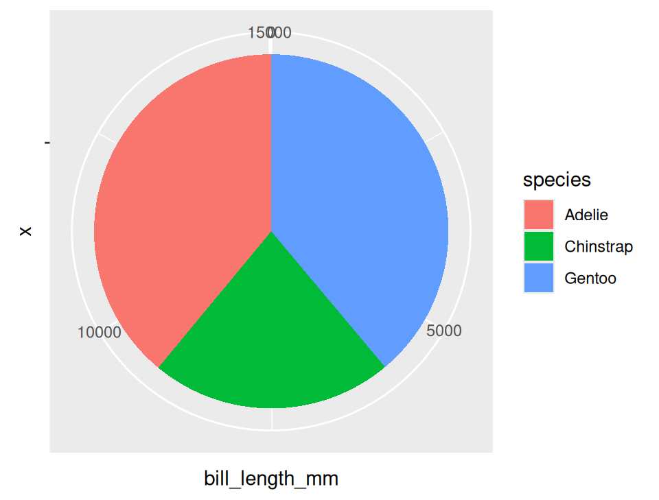
Coordinate Systems
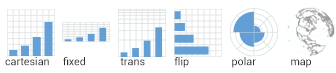
coord_cartesian(xlim=c(2,8))for zooming incoord_mapfor controlling limits on mapscoord_polarfor polar cordinates
Theming
- Modify non-data plot elements/appearance
- Axis labels, panel colors, legend appearance etc
- Save a particular appearance for reuse
?theme
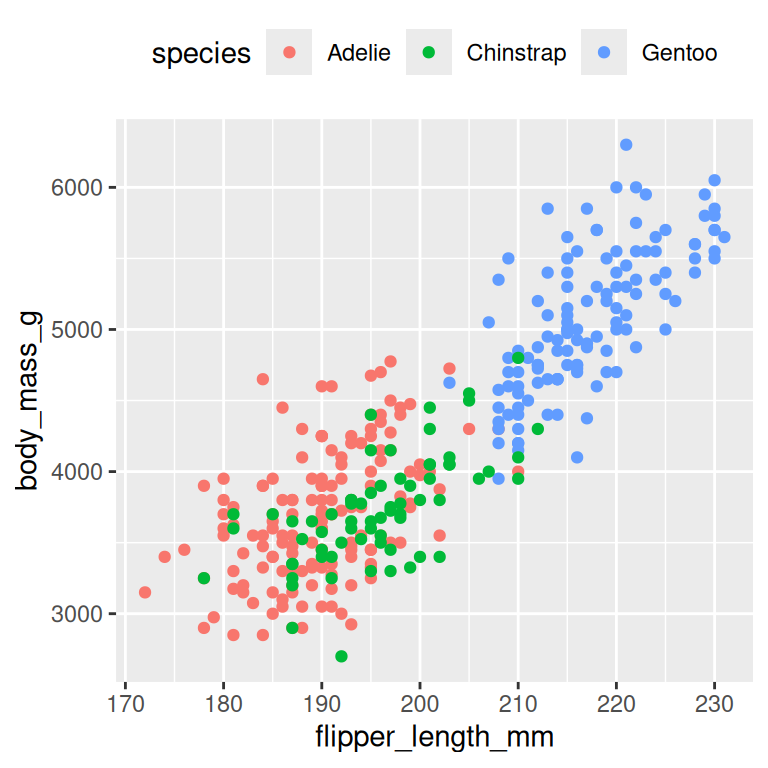
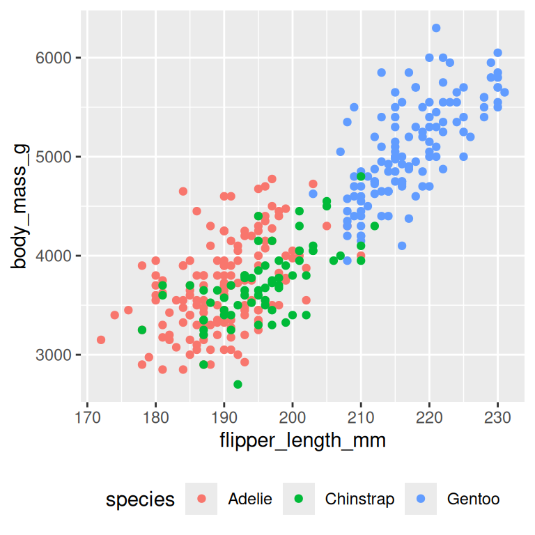
Theme • Legend
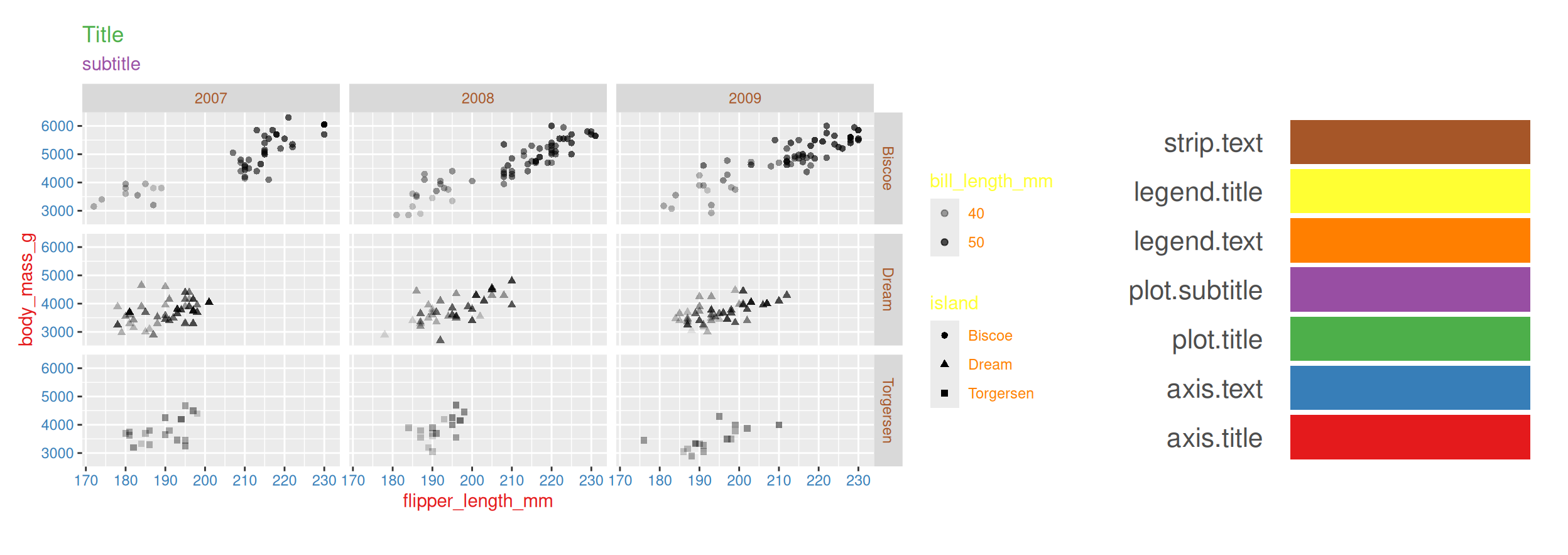
Theme • Text
Theme • Text
p <- p + theme(
    axis.title=element_text(color="#e41a1c"),
    axis.text=element_text(color="#377eb8"),
    plot.title=element_text(color="#4daf4a"),
    plot.subtitle=element_text(color="#984ea3"),
    legend.text=element_text(color="#ff7f00"),
    legend.title=element_text(color="#ffff33"),
    strip.text=element_text(color="#a65628")
)
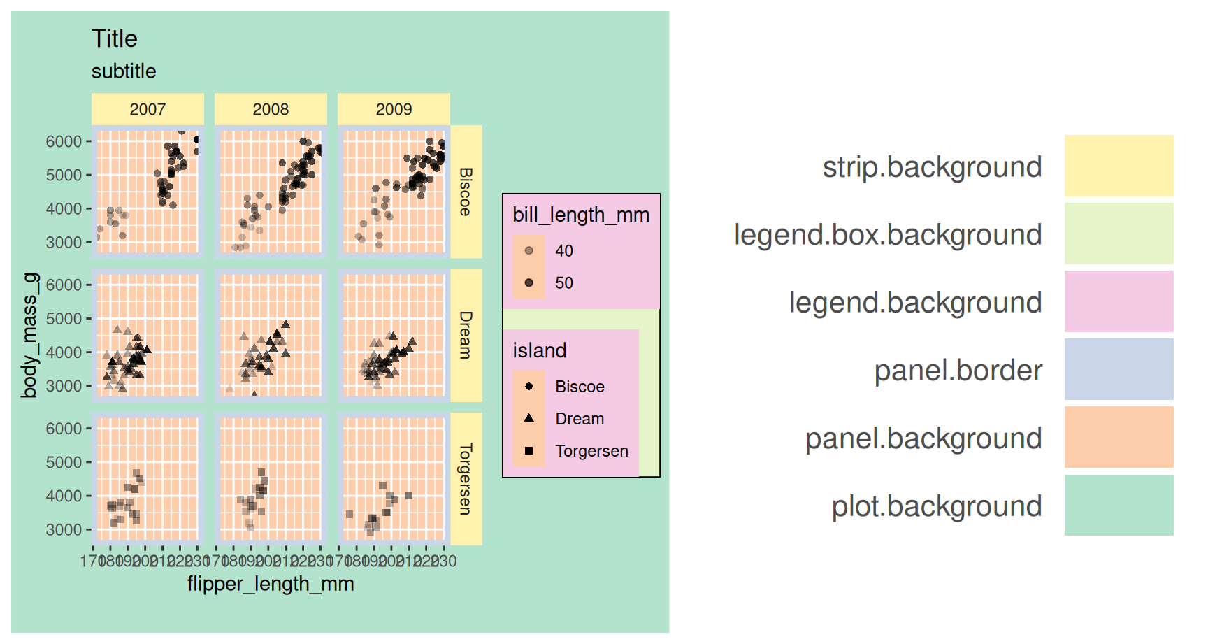
Theme • Rect
p <- p + theme(
    plot.background=element_rect(fill="#b3e2cd"),
    panel.background=element_rect(fill="#fdcdac"),
    panel.border=element_rect(fill=NA,color="#cbd5e8",size=3),
    legend.background=element_rect(fill="#f4cae4"),
    legend.box.background=element_rect(fill="#e6f5c9"),
    strip.background=element_rect(fill="#fff2ae")
)
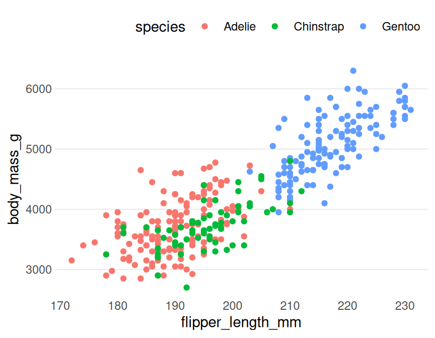
Theme • Reuse
newtheme <- theme_bw() + theme(
  axis.ticks=element_blank(), panel.background=element_rect(fill="white"),
  panel.grid.minor=element_blank(), panel.grid.major.x=element_blank(),
  panel.grid.major.y=element_line(size=0.3,color="grey90"), panel.border=element_blank(),
  legend.position="top", legend.justification="right"
)
Professional themes
Saving plots
ggplot2package offers a convenient function
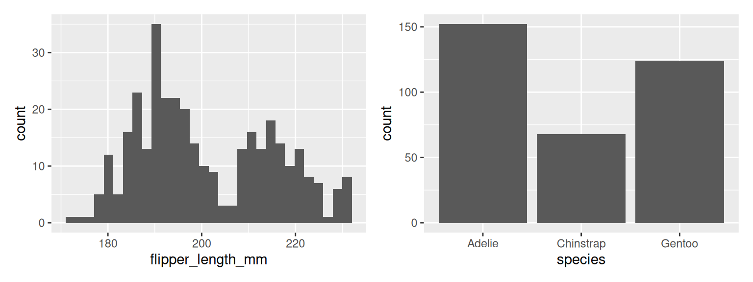
Combining Plots
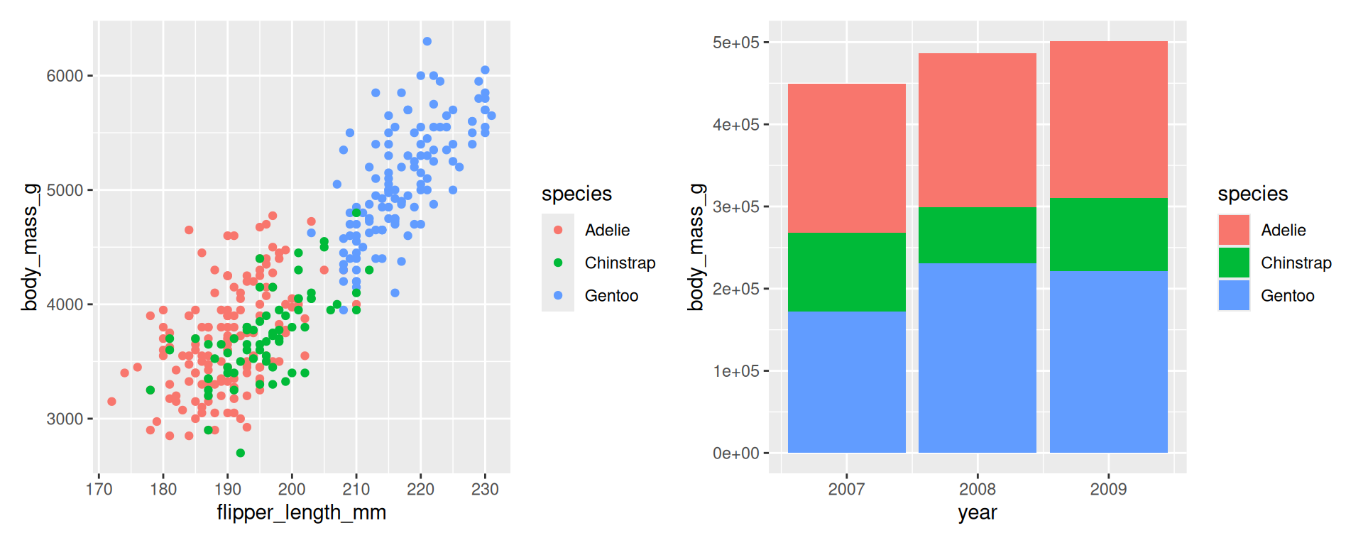
Combining Plots
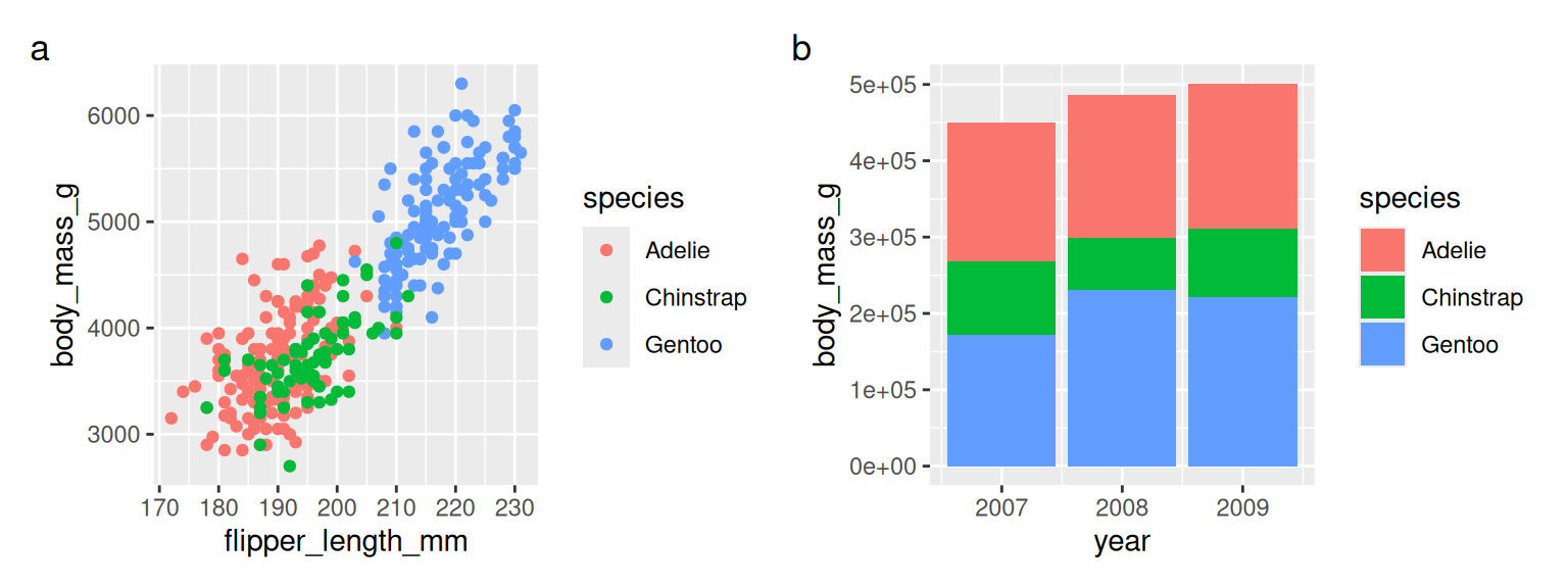
patchwork documentation.
Help
Thank you! Questions?
Acknowledgements:
• SLUBI • 3Bs • Slides adapted from RaukR • GPL-3 License